
Systems of Linear Equations: UPSC Mathematics Optional: Teacher’s words to prepare in right way
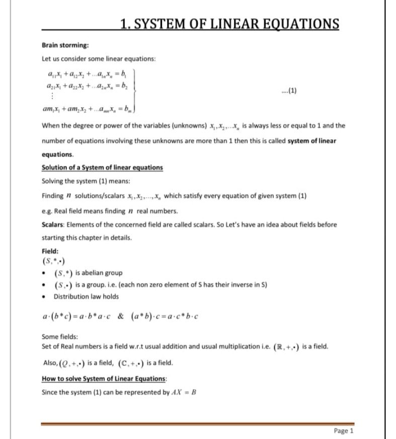
Let’s say I have given you some equation, and then I give you another one. Why have I written this? Because our childhood was like this, when we grew up we got here, and today we are going to get here. What is the target? When you were young, your teacher said, “Solve this equation.” You used to think these were just equations. Now that you have grown up, you are told that if you have more than one thing, you will call it a system of things.
Understand this carefully. Here we have two equations, so this is a system of two equations. There may be a system of three equations or a system of m number of equations, right? Understand my point carefully: this is a system of two linear equations, my dear fellows. When I use the word linear, it means whatever variables you are taking—x, y, z—their power is one. That is in linear form. If the powers of x and y are one, then it is called a linear equation. These variables whose values you want to find out are called unknowns.
So here we have a system of three linear equations in three unknowns. And in general, we have m linear equations in n unknowns—whatever unknowns we have, from \(x_1\) to \(x_n\).
What Does Solving a System Mean?
Understand it carefully: “Solve the given system of linear equations.” What is the meaning of this, my dear fellows? The meaning is to find the values of the unknowns that satisfy each of the given equations. The simple meaning of solving the system is just this.
Now, look at how your childhood was spent, friend. You used to multiply equation one by two, subtract it from equation two, and eliminate a variable. In three equations, you used to eliminate x and y and then solve it. But that childhood method is not useful here. Why will we not do it that way? Because up to three unknowns and three equations, it is fair enough. But when you have 100 unknowns and 150 equations, how can you do that manually? Are you getting my point? That is not possible manually. In that case, you have to develop some algorithm. A systematic approach will have to be developed so that whatever the number of unknowns in the equation, you feed that in and get your answer.
Matrix Representation: AX=B
To do this, observe this system carefully. This system can be represented in the form of a matrix if I take the coefficients, and I hope you know how to multiply two matrices, right? If you observe, x+2y=2 and the second equation can be written in matrix form. Similarly, if you observe the three-equation system, this will be written as a 3×3 matrix multiplied by the column of x,y,z equal to the right-hand side.
AX=B ; x+y=2, 2x-y=1
So here we will have \(x_1, x_2, \dots, x_n\) on the left, and it goes to \(b_1, b_2, \dots, b_m\) on the right. This means a system of linear equations can be represented like this.
If I call this coefficient matrix capital A, if I call this unknown column vector capital X, and if I call this right-hand side column capital B, then what we have discussed till now is that whenever we are given a system of linear equations, it can always be reflected in the form:
AX=B
Is everything clear till here? Here, A is called the coefficient matrix, X is the unknown vector, and B is the constant or RHS vector. Note that if B is a zero matrix, the system reduces to AX=0 and is called a homogeneous system of linear equations; if \(B \neq 0\), it is called a non-homogeneous system.
Demand-Driven Learning and Elementary Row Operations
Now understand carefully how we solve it. See, the story is the same as that of childhood, just a little bit more systematic here. Suppose you want to solve this system AX=B. Basically, we try to reduce A into a simpler form. Look, first we will create the demand, and then we will see why this topic is being read. The right way to learn anything is just like a child.
If I ask you what you did to solve the equations in childhood, you multiplied an equation by two and subtracted it, which ultimately eliminated x from the second equation. You got something in a simpler form. Now, when you multiplied everything in each equation, you have to give that step a formal name; only then can you develop a systematic approach.
We do this by applying row and column operations. Traditionally, we mainly work with row operations. It is not the case that we cannot do it with columns—we can—but row operations are traditional in this work, so we will go with that. That is why we said learning should be demand-driven. Now we have come to Elementary Row Operations.
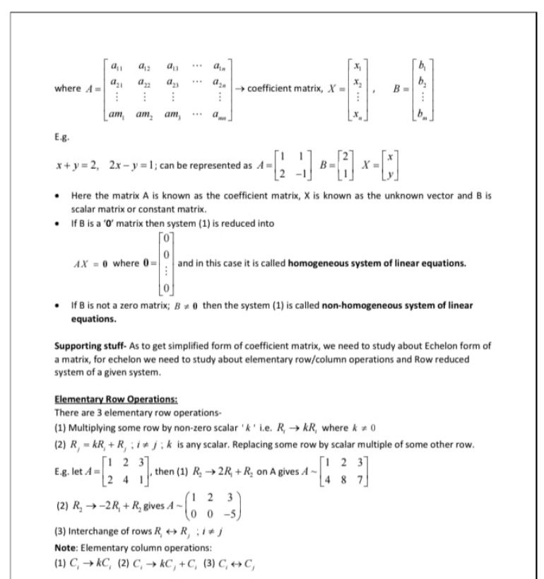
My dear fellows, there are three elementary row operations. Understand what those are:
1. Scaling a Row
If I replace the i-th row (whether it is the first, fourth, fifth, or tenth row) by k times that row, where k is a non-zero scalar:
\(R_i \rightarrow kR_i (k \neq 0\))
When you do that with a matrix, this is called an elementary row operation. Suppose we are working on AX=B. When you multiplied an equation by two in childhood, you did not just multiply the left side; you worked with the coefficients and also the things available in the RHS. So basically, you write an augmented matrix where you apply the operation on the coefficients and simultaneously operate on what is available in the RHS. For example, if I say \(R_1 \rightarrow 2R_1 \) we multiply the first row by 2 and keep the second row as it is. This is the first elementary row operation.
2. Adding a Multiple of One Row to Another
Now I move on to the second elementary row operation. Understand carefully what it does. I replace the j-th row by adding k times the i-th row to the j-th row, where k is non-zero and \(i \neq j\):
\(R_j \rightarrow R_j + kR_i \ (k \neq 0, i \neq j\)
You might be wondering what this means. For example, \(R_2 \rightarrow R_2 – R_1\). You used to do the exact same thing in your childhood! You might say, “Sir, there is subtraction in maths, why are you writing addition?” Well, in maths, there are really only addition and multiplication, and subtraction is just adding the additive inverse. So basically, the work is the same as multiplying equation one by two and subtracting it from equation two, but to formalize that, we write it like this. So the first row remains unchanged, and \(R_2\) is operated on to produce zeros below the first entry.
3. Interchange of Rows
The third elementary row operation is the interchange of rows:
\(R_i \leftrightarrow R_j\)
Look, we had a habit in childhood—I don’t know whether it was yours or not—that suppose I am given some equations, and one of them has a leading coefficient of 1. I felt happier solving the system by making that equation number one. So what I mean to say is you can freely interchange any two rows to bring a simpler equation to the top.
Study Complete Linear Algebra With Mindset Makers Academy
Want to master every categorical example, Echelon Form reduction, and 26 years of UPSC CSE & IFoS Previous Year Questions in this exact step-by-step sequence?
- Get the Complete 16+1 Core Literature Book Set: Systematically typeset physical volumes covering Theory, Categorical Examples, 26-Year Chapter-Wise PYQs, and Short Revision Notes. Explore the 16+1 Books →
- Join the 2027 & 2028 Evaluation Tracks: Practice answer writing under strict Sunday schedules with 48-hour copy evaluations and final macro audits by Prof. Upendra Singh. View Test Programs →